Types of ETL Transformations
2020-05-31
4 minutes
In ETL, I’ve found that most people think of the “transform” step as just a simple transformation on the new data. This might be the case if you’re converting variable types or applying simple row-wise transformations. But it’s more nuanced than that, particularly when your transformations are aggregations. In my experience, I’ve found three common types of transformations that take place. My loose categorization for them is historical, new data, and sliding window transformations.
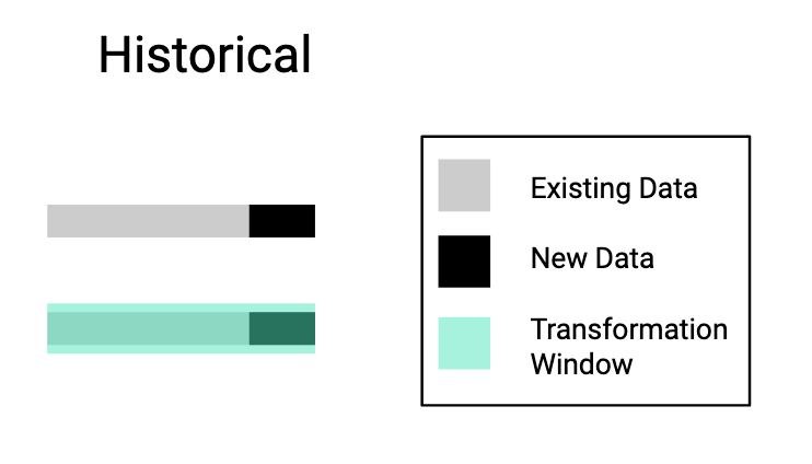
Historical
In historical transformations you’re applying a transformation over the entire history of data after the new data comes in.
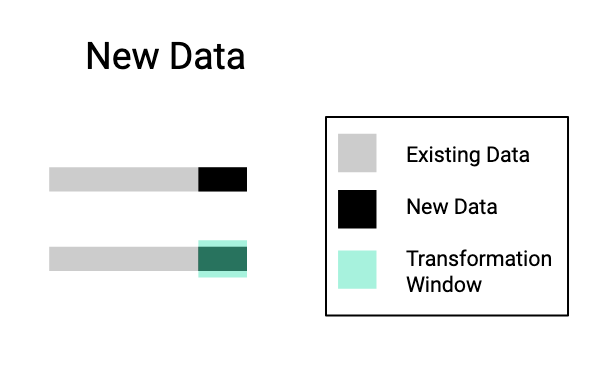
New Data
With new data transformations you’re applying a transformation to only new data coming in.
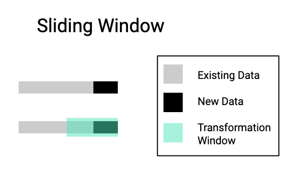
Sliding Window
With sliding window transformations you’re apply a transformation to the new data and to a subset of the history.
Useful Tricks
Implementing transformations in practice can be challenging. Instead of just dealing with the transformation itself you’re responsible for making sure that it is applied on some cadence. This is particularly problematic when trying to make sure code runs efficiently over large amounts of data.
With new data transformations the update pretty much takes care of itself, provided that the new data coming in is small enough. With historical and sliding window transformations the updates can be time consuming (even simple ones) if you don’t make them efficient.
Updating Historical
Suppose we want to keep some sort of historical aggregation up-to-date. For example, we want to maintain a table that tells us how many hours each user has spent watching movies using a streaming service platform. (Assume that the data we have available records how long each user has spent watching each movie, and that this data updates daily.) One approach to solve this would be,
- read in all of the data
- group by users
- sum the column that records time spent watching movies.
This is pretty inefficient (even if we stored data in a columnar format) since we have to read in all of the historical data as well as the new data to compute the sum.
A more efficient approach would be to first do a one-off historical backfill of the user-level sum (defined in steps 1-3) using all of the historical data to date. Then as the new data comes in we implement the summation aggregation (defined in steps 1-3) only on the new data. Finally, since we’re dealing with summation, we can simply add the new data aggregation with the historical aggregation (at the user-level of course).
Each time this is scheduled to run we’re only running transformations on the new data rather than all of the data, making this approach way more efficient. This approach basically computes the information of a “historical” transformation but did it with the efficiency of a “new data” transformation.
Updating Sliding Window
You have to be a bit more creative when trying to keep sliding window transformations up-to-date. Suppose we want to create the same table described above. Now instead of applying a transformation over the full history of user behavior we want to do it over a 1 week window.
A simple approach would be to do the 1 week transformation every time new data comes in. But with large data this can be infeasible.
If we follow the steps in the previous section, we get the new data aggregation (which is 1 day’s worth of data) and the historical aggregation (which, in this case, is 1 week’s worth of data). Summing them gives us 8 days worth of data. We still need to drop the first day that comes with the historical aggregation. Since we’re dealing with sums, we can do this by calculating the aggregation for just first day and subtract it from the sum of the new data aggregation and the historical aggregation.
This is more efficient since we’re applying transformations over only two time intervals (in this case days) of data; the first day and the latest day. Both these time intervals combined are smaller than applying the transformation over a week of data.
671 Words